analtech

How to Analyze Circuits in the Time Domain

July 27, 2025

← Prev Next →

Why “time‑domain (piecewise) circuit analysis” matters

When a switch flips, a source steps, or a waveform changes shape, your circuit’s differential equations also change. Time‑domain (piecewise) analysis is about tracking each interval, enforcing initial conditions at the switching instants, and stitching the responses together.

Core ideas you must keep in your head

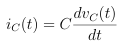
1. Initial Conditions

Capacitor voltage and inductor current are continuous:

$v_C(0^+) = v_C(0^-), \quad i_L(0^+) = i_L(0^-)$

2. Natural vs. Forced Response

Natural Response: what the circuit does when all independent sources are turned off.
Forced Response: specific response to external sources.

The total response is:

$x(t) = x_n(t) + x_f(t)$

3. First‑Order Time Constants

RC circuit:

$\tau = RC$

RL circuit:

$\tau = \frac{L}{R}$

General solution:

$x(t) = x(\infty) + \left[x(0^+) - x(\infty)\right] e^{-t/\tau}$

4. Second‑Order (RLC) Damping

Define:

$\alpha = \frac{R}{2L}, \quad \omega_0 = \frac{1}{\sqrt{LC}}, \quad \zeta = \frac{\alpha}{\omega_0}$

If $\zeta < 1$ → underdamped
If $\zeta = 1$ → critically damped
If $\zeta > 1$ → overdamped

Underdamped frequency:

$\omega_d = \sqrt{\omega_0^2 - \alpha^2}$

Quick “cheat sheet” formula

First‑order response:

$x(t) = x(\infty) + \left[x(0^+) - x(\infty)\right] e^{-(t - t_0)/\tau}, \quad t \ge t_0$

Second‑order (underdamped) step response:

$v_C(t) = V_{\text{step}} \left[1 - e^{-\alpha (t - t_0)} \left( \cos(\omega_d (t - t_0)) + \frac{\alpha}{\omega_d} \sin(\omega_d (t - t_0)) \right) \right]$

🧪 Example 1 (Beginner): RC Step Response

Given:
R = 10 kΩ, C = 0.1 μF, Step input: 5 V at t = 0, initially uncharged.

Time constant:

$\tau = RC = (10^4)(0.1 \times 10^{-6}) = 10^{-3} , \text{s}$

Initial & final voltages:

$v_C(0^+) = 0, \quad v_C(\infty) = 5 , \text{V}$

Voltage across the capacitor:

$v_C(t) = 5\left(1 - e^{-t/\tau} \right) = 5\left(1 - e^{-t/1\text{ms}} \right)$

🧪 Example 2 (Intermediate): RL Step Change

Given:
L = 0.1 H, R = 20 Ω, DC step from 10 V → 20 V at t = 0.

Initial current (steady state before switch):

$i_L(0^+) = i_L(0^-) = \frac{10}{20} = 0.5 , \text{A}$

Final current:

$i_L(\infty) = \frac{20}{20} = 1 , \text{A}$

Time constant:

$\tau = \frac{L}{R} = \frac{0.1}{20} = 5 , \text{ms}$

Current response:

$i_L(t) = 1 + (0.5 - 1) e^{-t/\tau} = 1 - 0.5 e^{-t/5\text{ms}}$

🧪 Example 3 (Advanced): Underdamped RLC

Given:
Series RLC: R = 10 Ω, L = 0.1 H, C = 100 μF, Step input 10 V at t = 0, initially relaxed.

Damping factor:

$\alpha = \frac{R}{2L} = \frac{10}{0.2} = 50 , \text{s}^{-1}$

Natural frequency:

$\omega_0 = \frac{1}{\sqrt{LC}} = \frac{1}{\sqrt{0.1 \cdot 1 \times 10^{-4}}} \approx 316.23 , \text{s}^{-1}$

Damped frequency:

$\omega_d = \sqrt{\omega_0^2 - \alpha^2} \approx \sqrt{316.23^2 - 50^2} \approx 312.25 , \text{s}^{-1}$

Capacitor voltage response:

$v_C(t) = 10 \left[1 - e^{-50 t} \left( \cos(312.25 t) + \frac{50}{312.25} \sin(312.25 t) \right) \right]$

🧾 Summary Checklist for Time-Domain Solving

Determine initial conditions:

$v_C(0^-), \quad i_L(0^-)$

Enforce continuity:

$v_C(0^+) = v_C(0^-), \quad i_L(0^+) = i_L(0^-)$

Compute final value
$x(\infty)$ for each interval

Apply template for solution: first or second order

25_07_27 Download

Understanding Mixed DC–AC Circuits the Easy Way

How to Calculate Charging Time in RC Networks

← Prev Next →

kds881119

IF YOU WANNA READ DAILYNEWS CLICK HERE

Leave a Reply Cancel reply