
Mastering Kirchhoff’s Current Law (KCL): A Guide for Intermediate Learners
In the world of circuit analysis, Kirchhoff’s Current Law (KCL) is not merely a starting point—it’s a crucial tool for accurately modeling, analyzing, and troubleshooting electrical networks. While beginners might use KCL to solve basic series-parallel networks, intermediate-level engineers apply it systematically to multi-node systems, especially when designing embedded systems, power electronics, and analog signal chains.
This post dives deeper into how KCL works, explores real-world cases, and introduces effective techniques to apply the law in more complex scenarios.
The Law Behind Current Conservation
KCL is based on a fundamental principle in physics: the conservation of electric charge. In electrical circuits, this translates to the following statement:
At any node (junction) in an electrical circuit, the algebraic sum of currents entering and exiting that node must equal zero.
This can be written as:
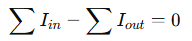
Or, rearranged more practically:

Where current entering is considered positive and current leaving is negative (or vice versa, depending on your sign convention—consistency is key).
KCL in Multi-Node Circuits
In a typical circuit with several components and nodes, KCL allows you to write one current equation per independent node. Consider a node connected to three resistors with currents I1, I2, and I3:
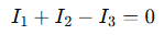
This equation is valid regardless of the complexity of the components—as long as you define the current direction consistently. In intermediate-level problems, KCL is typically paired with Ohm’s Law and KVL (Kirchhoff’s Voltage Law) to solve unknowns using nodal analysis.
Example: Three-Node Resistive Circuit
Let’s analyze a simple circuit to demonstrate KCL in action.
Circuit Description:
- Node A connects three branches:
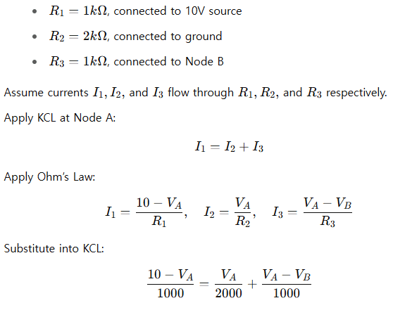
This equation is solvable using algebra or matrix methods when combined with other KCL equations for other nodes.
Techniques for Efficient Node Analysis
1. Label Nodes Clearly

2. Assume Current Directions
Even if guessed incorrectly, the solution will return negative current values—which still makes sense.
3. Use Conductance (G = 1/R)
Converting resistances to conductance simplifies matrix formation for large circuits.
4. Formulate a Matrix
Use the node-voltage method to build a system of equations:

This becomes essential in SPICE simulations and algorithmic analysis.
Common Pitfalls for Intermediate Users
- Skipping Reference Node: Always define ground or 0V reference.
- Redundant Equations: Writing too many KCL equations may result in dependent equations.
- Mixing KCL and KVL Inconsistently: Avoid combining methods with mismatched sign conventions.
KCL Beyond Resistive Networks
KCL also applies in capacitive and inductive circuits, albeit with time-dependent current equations.
Capacitor Node Example:
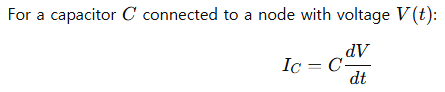
KCL becomes a differential equation:
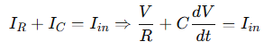
This is the basis of first-order system modeling in control systems and analog filters.
Applications in Engineering Systems
- Analog Signal Processing: Node current control in operational amplifiers
- Power Systems: Balancing load currents at distribution points
- Digital Systems: Ensuring proper current sourcing in FPGA logic blocks
- PCB Design: Avoiding current overflow at high-speed nets
In each domain, mastering KCL ensures not just design correctness but system stability and efficiency.
Conclusion
Kirchhoff’s Current Law remains one of the most powerful and reliable tools for engineers engaged in electrical design. At the intermediate level, its application goes far beyond simple current addition—it becomes a stepping stone to modeling, simulating, and validating circuits under real-world constraints.
By combining KCL with Ohm’s Law and systematic node analysis, you can tackle complex networks with clarity and confidence—whether on paper or in simulation software.
Leave a Reply