
Advanced KCL Techniques for High-Fidelity Circuit Analysis
In advanced electrical engineering, Kirchhoff’s Current Law (KCL) is no longer a basic identity—it becomes a strategic tool for high-accuracy analysis of complex, time-variant, and nonlinear systems. Beyond the basic “sum of currents equals zero” idea, engineers use KCL in a wide range of analytical domains: differential system modeling, node-voltage matrix solving, fault detection, power distribution analysis, and embedded analog design. This article explores how professionals deploy KCL at an advanced level to solve real-world engineering challenges with mathematical rigor.
1. Revisiting KCL from a Theoretical Standpoint
KCL is a direct consequence of the continuity equation derived from Maxwell’s equations. It assumes that charge cannot accumulate instantaneously at any point in a steady-state circuit. In integral form:
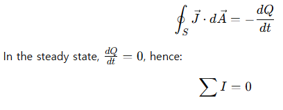
This makes KCL valid under the assumption that displacement currents and distributed parameters can be neglected, which is generally true for lumped-element circuits operating well below GHz frequencies.
2. Node-Voltage Method Using KCL
In large-scale resistive networks, KCL forms the basis for the nodal analysis method, yielding a system of linear equations:
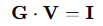
Where:
- G: Conductance matrix (derived from inverse resistance values)
- V: Vector of node voltages
- I: Source current vector
For example, a 4-node network will generate a 3×3 linear system (excluding reference ground node). LU decomposition, Gauss-Seidel iteration, or matrix inversion methods are then applied.
This matrix formalism becomes essential when transitioning to SPICE or symbolic computation environments like MATLAB or Python’s SymPy.
3. KCL in Time-Domain: Differential Equations and Laplace Transform
For dynamic circuits including capacitors and inductors, current becomes time-dependent, making KCL yield differential equations. Consider a capacitive node:
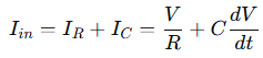
Applying Laplace Transform for frequency-domain analysis:
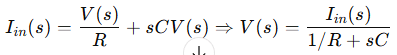
This transformed KCL equation is used in designing analog filters, control systems, and feedback amplifiers.
4. KCL in Nonlinear Systems
When analyzing nodes connected to nonlinear elements such as diodes, BJTs, or MOSFETs, KCL becomes an implicit equation system:

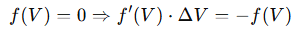
These systems require iterative methods like Newton-Raphson or Broyden’s method for convergence. Solvers typically start with a linearized model:
This is the backbone of modern EDA (Electronic Design Automation) simulators, where KCL equations must be solved with high numerical stability and precision.
5. Practical Use Cases in High-Performance Systems
a. Mixed-Signal IC Design
KCL ensures current matching at sensitive analog input nodes to prevent distortion in ADCs and DACs.
b. Power Electronics
Current balancing in DC-DC converters, H-bridge circuits, and inverter topologies rely on precise KCL application across fast-switching MOSFETs and IGBTs.
c. Telecom and RF Systems
KCL is applied in impedance-matched networks where even nanoampere errors at high frequency can cause VSWR (Voltage Standing Wave Ratio) instability.
6. Common Pitfalls and Precision Strategies
- Floating Nodes: Always tie unused nodes to known references to prevent undefined behavior.
- Numerical Round-off: Use high-precision libraries for matrix solutions, especially in ill-conditioned systems.
- Model Abstraction Error: Simplifying distributed networks into lumped elements may invalidate KCL in GHz or mmWave domains. Use full-field EM solvers when necessary.
7. Beyond Circuit Theory: KCL in System Modeling
KCL analogs are used in:
- Neural Engineering: Modeling ion channel currents in Hodgkin-Huxley equations
- Thermal Networks: Applying KCL analog for heat flow analysis (temperature ↔ voltage, thermal resistance ↔ electrical resistance)
- Fluid Dynamics: Mass conservation in node-pipe networks, interpreted through KCL’s framework
Conclusion
For high-fidelity electrical design, mastering KCL goes beyond textbook usage. It requires a deep understanding of physical laws, numerical methods, dynamic modeling, and system-level implications. Whether you’re designing low-noise amplifiers or modeling control loops in a converter, KCL remains a foundational but profoundly powerful principle.
Applying it with mathematical rigor and system awareness unlocks precise, reliable, and innovative circuit solutions in every domain of modern electronics.
Leave a Reply