
Kirchhoff’s Voltage Law (KVL) may be one of the first principles taught in circuit theory, but its utility extends well into advanced electrical engineering. For seasoned engineers and graduate students, KVL is not merely a conceptual tool — it is foundational in linear circuit analysis, network theory, and numerical modeling.
In this post, we will explore KVL from a higher-level analytical standpoint, with a focus on complex impedance, mesh matrix formulation, and its role in modern simulation and control systems.
1. Revisiting KVL in Formal Terms
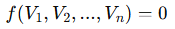
KVL is derived from the conservation of energy and is expressed in its most general form as:
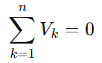
for any closed path (mesh) in a circuit, where VkV_kVk is the voltage across element k.
This implies that as we traverse a loop in the circuit, the algebraic sum of electromotive forces (EMFs) and voltage drops due to passive elements is zero.
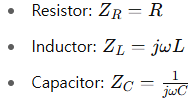
2. KVL in the Complex Frequency Domain
In real-world circuits, components exhibit frequency-dependent behavior. KVL still applies, but voltages and currents are now treated as phasors and elements are represented by complex impedance:
KVL equations in AC steady-state become:
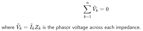
This formulation is essential in designing and analyzing resonant circuits, filters, and matching networks in RF and signal processing.
3. Mesh Analysis Using Matrix Formulation
For large-scale linear systems, matrix-based mesh analysis is the most efficient method to implement KVL. Consider a system with m meshes. Define:
- Z: mesh impedance matrix
- I: mesh current vector
- V: source voltage vector
The system of equations derived from KVL is:

Where each row corresponds to one mesh equation. This compact representation enables the use of numerical solvers in tools like MATLAB, Python (NumPy), or SPICE simulators.
4. Handling Dependent Sources and Controlled Elements
In advanced network theory, voltage-controlled and current-controlled sources are common. KVL must account for such elements by expressing their voltage drops as functions of other currents or voltages.
For example, in a loop containing a voltage-controlled voltage source (VCVS):
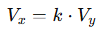
This constraint must be substituted into the KVL equation accordingly, increasing the system’s complexity but preserving linearity.
5. Application in Nonlinear and Time-Varying Circuits
Though KVL is strictly valid under lumped circuit assumptions, it can still be extended to nonlinear or time-varying circuits if voltages are defined across identifiable elements.
For circuits involving diodes, transistors, or nonlinear inductors, KVL equations take the form:
This typically requires solving nonlinear algebraic or differential equations numerically.
In switched-mode power supplies (SMPS) and PWM-controlled circuits, KVL is applied piecewise within each switching state, combined through state-space averaging or Fourier analysis.
6. Integration with Modified Nodal Analysis (MNA)
While KVL is traditionally loop-based, in large system simulations, nodal methods are often preferred. However, Modified Nodal Analysis still embeds KVL indirectly via:
- Loop constraints
- Branch relationships
In matrix terms, the loop constraints can be represented using the incidence matrix A and loop matrix B:

Here, v is the branch voltage vector. The entire circuit solution thus integrates KVL, KCL, and constitutive relations.
7. Real-World Use Cases of Advanced KVL
- Power system analysis: In load flow and fault studies, KVL is used to derive bus voltages in multi-node networks.
- Analog circuit design: Op-amp stability, feedback path modeling, and gain calculation often rely on precise loop analysis.
- Control systems: In modeling electric machines or actuators, KVL-based models help form dynamic equations for motor drives.
- Signal integrity in PCB design: Loop impedance calculations are essential for minimizing noise and reflection in high-speed digital circuits.
8. Final Thoughts: KVL Beyond the Basics
Kirchhoff’s Voltage Law is more than just a fundamental rule — it is a structural principle of all lumped-parameter electrical systems. Whether working in the frequency domain, building large-scale simulations, or designing hybrid analog-digital systems, KVL remains indispensable.
Understanding its advanced applications ensures you can move confidently through:
- Linear and nonlinear system analysis
- Time-domain and frequency-domain modeling
- Symbolic and numerical simulation environments
In the evolving landscape of electronics and embedded systems, mastery of KVL at this level is not optional — it’s essential.
Next Step: Explore how KVL works hand-in-hand with state-space modeling and Laplace-domain analysis to represent entire system dynamics, especially in control and automation.
Leave a Reply